Ionosphere : Tutorial
Contents
2 Ionospheric Activity
3 Ionospheric Refraction, Phase Delay and Total Electron Content
4 How to Mitigate the Ionospheric Refraction ?
5 How to Estimate the Total Electron Content from GPS Data ?
6 How to Convert STEC in VTEC ?
7 How to Obtain a 4D Image of the Electron Concentration of the Ionosphere ?
7 Ionospheric products
8 Halloween Storm
9 Bibliography
What is the Ionosphere ?
History
1861: [Stewart, 1861] linked the abnormal magnetograph observations at the Kew observatory for the period August-September 1859 with the large sunspots observed in the same time by Carrington. This is the first study on the impact of the solar activity on the earth magnetosphere. This event, called the Carrington event, is at the origin of the space weather research.
1889: [Schuster, 1889] advanced the hypothesis that a conducting region should exist in the upper atmosphere to explain diurnal variations of the geomagnetic field.
1902: Heaviside and Kennelly explained the propagation of radio waves over long distances by the presence of a reflective shell in the upper atmosphere.
1925: The existence of ionised regions in the upper atmosphere was proved by Appelton. He used the travel time of a radio signal from the BBC to estimate the lower altitude (~ 100km) of the Appelton shell.
1926: [Breit and Tuve, 1926] used an electromagnetic pulse to prove the existence of echoes from the upper atmospheric region. The effective height of the layer is between 80 and 210 km.
1929: Watson-Watt introduced the term ionosphere to define the ionised shell around the Earth to replace term Appelton layer.
1931: Chapman elaborates his theory on the ionization of layers by UV solar action.
Composition of the Ionosphere
The ionizing action of the sun's radiation on the Earth's upper atmosphere produces free electrons. Above about 60km the number of these free electrons is sufficient to affect the propagation of electromagnetic waves. This "ionized" region of the atmosphere is a plasma and is referred to as the ionosphere. [Rishbeth and Garriott, 1969] divided the ionosphere in to several layers:
D layer: 60 to 90 km; Pressure: 2Pa; Temp.: -76° C; electron concentration: 107-1010 e-/m3
Characteristics: D layer ionization is a function of the solar flow.
The ions are formed by the ionization of atmospheric neutrals by X-ray radiation and solar Lyman α radiation.
This region vanishes at night due to the combination of the ions
and electrons.
HF radio waves are not reflected
by this region, the main impact of which is absorption of high-frequency radio waves.
E layer: 90 to 150 km; Pressure: 0.01Pa; Temp.: -50° C; electron concentration: 1011 e-/m3
Characteristics: Similarly to the D layer, the E layer shows a diurnal behavior with a maximum of ionization at local noon.
In this region, ions consist primarily of O+2 produced by the absorption of solar radiation, and
NO+ formed by charge transfer collisions with other ions ionized by coronal X-rays. In auroral region, solar particle
precipitation can produce radio scintillation effects in the E layer.
F layer: 120 to 800 km; Pressure: 10-4Pa; Temp.: 1000° C; electron concentration: 1011 e-/m3
Characteristics: This layer is formed by ionization of atomic oxygen by Lyman emissions and emissions from He.
This region is sometimes divided into F1 and F2 sub-layers. The maximum electron concentration of the F1 region is close to 200km.
This layer, in which O+ ions transfer charge to neutrals to form NO+, disappears at night due to
dissociative recombination. The peak of the F2 layer electron concentration is at approximately 350km. In this layer, O+
remain the principal ion species. The F layer is the most important part of the ionosphere in terms of HF communications.
Ionospheric Activity
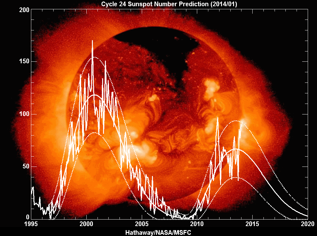
Figure 1: Sunspot number observed and predicted from 1995 to now.
The degree of ionization in the ionosphere depends essentially on the Sun, amount of radiation received from the Sun. Hence, there is a diurnal effect as the solar radiation received locally varies during the day.
There is a seasonal effect, since the local winter hemisphere is tipped away from the Sun, thus receiving less solar radiation. Different geographic regions of the Earth's surface (polar, auroral zones, mid-latitudes and equatorial regions) are also not equal with respect to the solar radiation they receive.
Moreover, the activity of the Sun follows the eleven-year sunspot cycle. Our star is more active and emits more radiation around maxima of the solar sunspot number.
Also, active solar phenomena such as solar flares are more frequent around solar maxima. Solar flares are associated with a release of charged particles into the solar wind. When the latter reach the Earth, it interacts with the Earth's geomagnetic field and causes some modification of the ionosphere. One sometimes speaks of a geomagnetic storm, a temporary intense disturbance of the Earth's magnetosphere, such as the one that occurred on the 30th October 2003.
Finally, recent researches show that earthquakes can affect the ionosphere by the propagation through the atmosphere of gravitational waves.
Ionospheric Refraction, Phase Delay and Total Electron Content
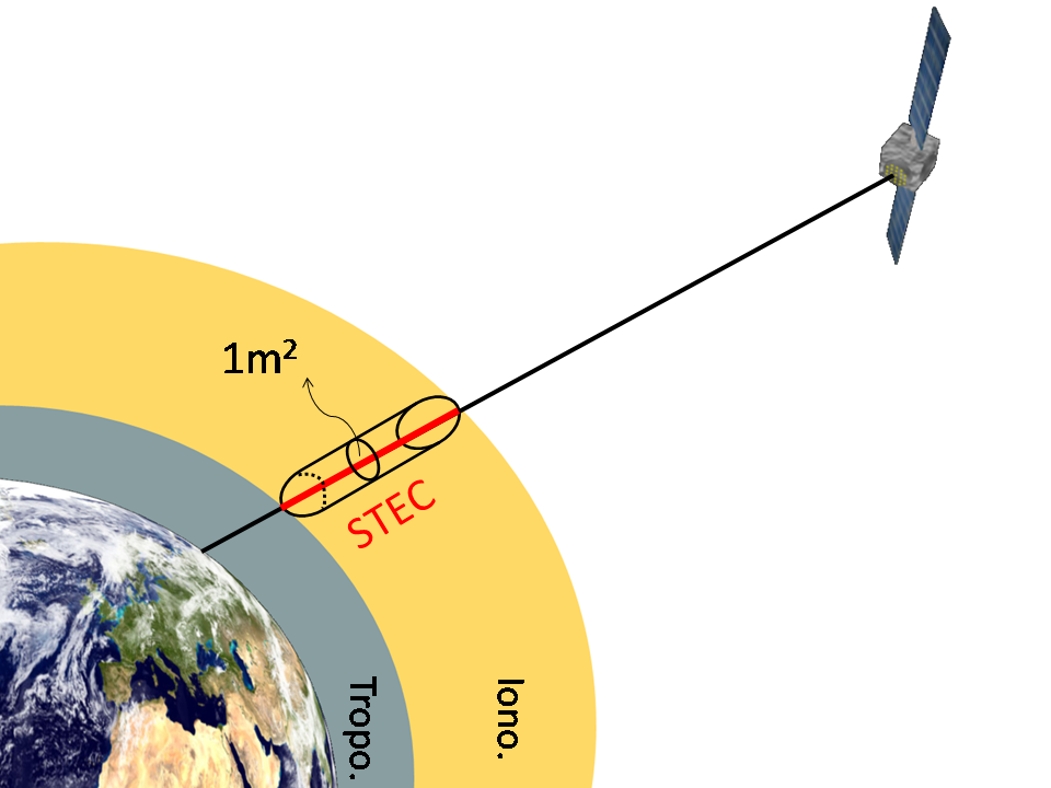
Figure 2: Slant Total Electron Content.
Electromagnetic wave signals are perturbed when travelling through the ionosphere. As the ionosphere is a dispersive medium, the ionospheric refraction depends on the signal frequency. The phase ionospheric refractive index is, to first order, given by:
with
where Ne is the number of free electron in the ionosphere (no free electrons in space or in the troposphere) between the receiver and the satellite and f are the GPS frequencies.
The effect of ionospheric refraction is to delay signal propagation. This causes a delay and advance for the GPS code and phase measurements respectively for the two GPS frequencies k=1,2:
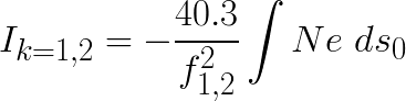
where s0 is the geometric range along the straight line between the satellite and the receiver.
The Slant Total Electron Content (STEC, Figure 2) is defined as the sum of Ne along the ray path:
where ds0 represents a cylinder of 1m2 cross-sectional formed around the ray path in which is assumed that all the electron content is concentrated.
The STEC is expressed in Total Electron Content Units (TECU):
According to the ionospheric refraction equation, the phase ionospheric delay is a function of the STEC:
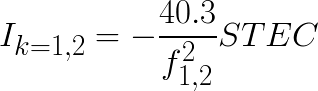
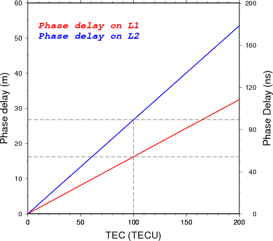
Figure 3: Phase delay in meters and nanoseconds with respect to the STEC.
The ionospheric refraction causes phase delays of the order of 16cm and 0.54ns for 1 TECU on the first GPS frequency phase signal (L1). Figure 3 give the phase delays on both GPS frequencies in terms of time and distance delays with respect to the STEC between a satellite and a receiver. Over Belgium the TEC can vary from 10 to 100 TEC or more.
The ionospheric refraction has a notable impact on the precise estimate of the GNSS receiver's position, or when performing time and frequency transfer between two stations equipped with precise clocks and GNSS receivers.
The ionosphere impact on GPS signals means a delay on the code and an advance on the phase measurements.
In addition to delays on GNSS signals, scattering of the GNSS radio signal by ionospheric irregularities may appear. These are called scintillations; they occur most frequently at tropical latitudes where it is a night-time phenomenon and less frequently at high latitudes or mid-latitudes except in the case of magnetic storms. These can affect GPS accuracy. Travelling Ionospheric Disturbances (TDIs) might also cause a loss of lock of the GPS signal (See Tutorial on How GNSS Works).
How to Mitigate the Ionospheric Refraction ?
For a given station, the GPS measurements, relative to the observed satellite, on the signal code P1,2 and phase φ1,2 , at the two GPS frequencies (f1=1575.42 MHz and f2=1227.6 MHz) with corresponding wavelength λ1,2 , can be written in length units as
where ρ1,2 is the geometric distance from the station to the satellite ; Δtrec is the station clock synchronization error; Δtsat is the satellite clock synchronization error; c is the speed of light velocity; Tr is the troposphere path delay for station; I1,2 are ionosphere delays on the two frequencies ; N are phase ambiguities; w1,2 are the phase windup ; δ1,2P are the hardware delays ; εP and εφ are the error terms in code and phase, containing noise and multipath (See Tutorial on Positioning and Timing).
The first order ionosphere effect, which amounts to 99.9% of the total ionosphere perturbation on GNSS signals, is proportional to the inverse of the square frequency. Hence, when dual frequency GPS receiver is available, the so called "ionosphere-free" combination of the two frequencies code and phase signal (P3 and L3 using the coefficient α and β) is used to remove thoroughly the first order ionosphere perturbation only:
and finally
The first order ionospheric perturbation is thus removed, but this combination is still affected by higher order ionospheric perturbations.
Concerning single frequency receivers, the user need an external information to correct the signal delay. For that, different methods can be used:
- The use of a network of nearby fixed stations with wellknown positions. The difference between the estimated and predicted position of those reference stations is due to the ionospheric and topospheric delays, the clock errors, the relativistic effect ... This information is transmitted to the single frequency user to correct its position. The main assumption of this method, called Differential Global Positioning System (DGPS), (See Tutorial on Positioning and Timing )), is to consider that the errors are the same for the reference stations and the single frequency station.
- The use of an external ionospheric model to correct the signal delay. Many models are now available: Global Ionospheric Maps, Klobuchar, IRI 2007 and the Nequick model. A description of these models is given at the end of this tutorial.
How to Estimate the Total Electron Content from GPS Data ?
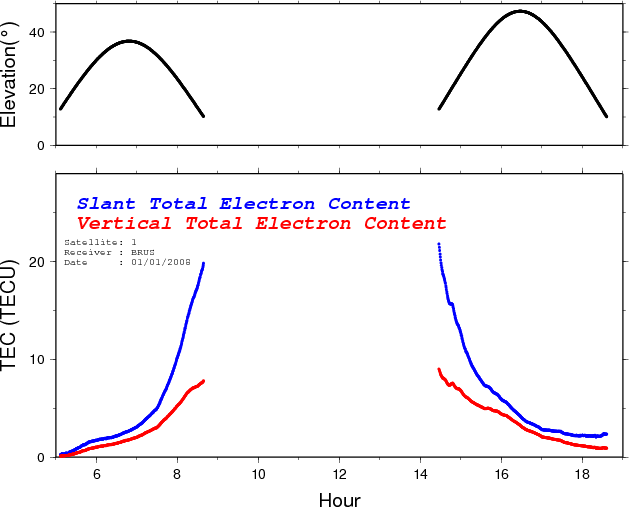
Figure 4: STEC and VTEC from satellite 1 and receiver BRUS, 1st January 2008.
To estimate the STEC between a satellite and a receiver, the delay between the phase and/or code measurements on the two frequencies is estimated using the geometry free combination P4 and Φ4:
where P1 or 2 and Φ1 or 2 are the code and phase observables are the two frequencies, Δbsat and Δbrec are the satellite and receiver differential inter-frequency hardware delay generally called Differential Code Biases (DCB), B4 is the phase ambiguity parameter, and I the ionospheric refraction linked to the Slant Total Electron Content (STEC) given in the previous equation.
Using these equations we can estimate the STEC between each satellite and each receiver.
How to Convert STEC in to VTEC ?
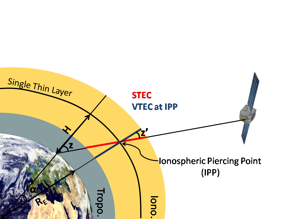
Figure 5: STEC vs VTEC.
The STEC depends on the length of the signal's path trough the ionosphere and is consequently dependant on the satellite elevation. To correct for this effect, an estimation of the Vertical TEC (VTEC) above a given point on the Earth surface is necessary. To determine this, the Single Thin Layer Model is usually employed. This model assumes that all the free electrons are concentrated in a layer of infinitesimal thickness located at the altitude H (figure 5).
The VTEC is estimated at each Ionospheric Pierce Point (IPP) from the ionospheric mapping function MFI according to figure 5:
with
How to Obtain a 4D Image of the Electron Concentration of the Ionosphere ?
Ionospheric imaging [Kunitsyn and Tereshchenko, 2003] is the representation of the electron concentration in the ionosphere in 4D (spatial and temporal dimensions). The technique uses tomographic principles to solve the inverse problem which consists to the determination of the electron concentration in the ionosphere (model) from the STEC estimations based on GNSS observations (data).
Figure 6: Representation of the direct problem. Reconstruction of STEC from the electron concentration.
To facilitate the understanding of tomography, let us consider a simple case representative of the direct problem which consists in calculating the STEC from the electron concentration. The ionosphere is schematically divided into 4 cells (Figure 6). In each of these cells there is a different electron concentration, Nek where k is the cell number. When a signal passes through a cell, the number of electrons encountered by the signal is the electron concentration of the cell multiplied by the length of the signal segment lk. Therefore the STEC is the sum of all segment lengths multiplied by their corresponding electron concentration.
Figure 7: Ionospheric tomography principle. Representation of a GNSS satellite which is emitting signals to receivers while is orbiting around the Earth.
The inverse problem reconstructs the electron concentration knowing the STEC and the segment length of the signal passing through the cells. In the case of figure 6, the retrieval of the electron concentration Nek is not possible due to the lack of STEC observations. However, by gathering a sufficient number of STEC data passing through the ionosphere, the electron concentration can be reconstructed by simultaneously solving a system of multiple STEC equations, each corresponding to a signal ray path.
Ionospheric imaging uses the same principles. The ionosphere is divided into cells and the STEC data are gathered from ground receiver networks. The use of large and dense receiver networks observing the maximum number of GNSS satellites is necessary to obtain a better scanning of the ionosphere in terms of spatial and temporal resolutions.
However as the number of observations gathered at a given time generally remains insufficient, the ionosphere is assumed to be in a stable state for a short time period. This assumption allows the use of multiple observations from each receiver-satellite pair during a few minutes to ensure a larger scanning of the ionosphere (Figure 7).
Despite of all this, it is not possible to generate straightforwardly a unique model solution of the ionospheric electron concentration due to the sparsity of the GNSS rays (too many electron concentration unknowns remain in the equation system) and the measurement errors in the STEC data. Therefore many options are used in ionospheric imaging to overcome this issue. First, other data can be added during the inversion: STEC data gathered from signals emitted from satellite to satellite or local measurements from ionosondes. Secondly, external ionospheric models (see the end of this tutorial) are used to improve the reconstruction. Finally, many different methods exist for ionospheric imaging [Bust and Mitchell, 2008] and have therefore different abilities to reconstruct the ionospheric model solution with a minimum error.
Ionospheric Products
The delays on radio signals travelling through the ionosphere are directly proportional to STEC. Consequently, single frequency users can correct for the ionospheric delay by TEC estimation. Several products are now available to estimate the TEC every where and at any time.
Global Ionospheric Maps (GIM): The International GNSS Service (IGS) Analysis Centre (http://igscb.jpl.nasa.gov/components/prods.html) provides VTEC maps. VTEC maps are global maps modelled by using up to 250 globally distributed GNSS stations and using TEC interpolation using spherical harmonics [e.g. Schaer et al, 1998]. These maps are estimated every two hours on a 2.5° /5° grid. Figure 8 presents an example of a global VTEC map at 12:00 UT on 21th March, 2009 form the CODE Analysis Centre Global Ionospheric Map (GIM), available at ftp://ftp.unibe.ch/aiub/CODE/)
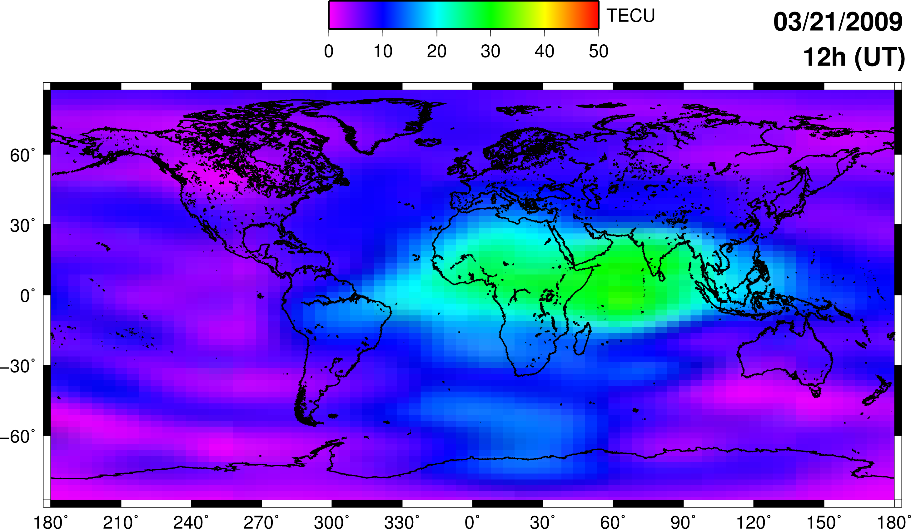
Figure 8: Global Ionospheric Map from CODE Analysis Centre.
Klobuchar model: The Klobuchar model [Klobuchar, 1987] is the broadcast Ionospheric Correction Algorithm (ICA) implemented in the GPS system. It is designed to correct for approximately 50% of the ionospheric range delay. It predicts the VTEC at a given time above a given location in order to correct for ionospheric delay in GPS measurements .
IRI 2007 model: The International Reference Ionosphere (IRI) (http://ccmc.gsfc.nasa.gov/modelweb/models/iri_vitmo.php) This model [e.g. Bilitza and Reinisch, 2008] is an empirical model based on a wide range of ground and space data. It gives monthly averages of electron density, ion composition (O+, H+,N+,He+, O+2,NO+ and Cluster+), ion temperature and ion drift in the altitude range 50-1500 km in the non-auroral ionosphere.
Nequick model: This empirical model has been proposed for use in making ionospheric corrections in the single frequency operation of the European Galileo project. It is a quick-run model that allows calculation of the electron concentration at any given location in the ionosphere and thus the Total Electron Content (TEC) along any ground-to-satellite ray-path by means of numerical integration [e.g. Hochegger et al., 2000].
Halloween Storm
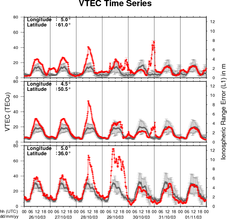
Figure 9: VTEC time series at 3 locations in Europe (North, Brussels, South) during the week around the geomagnetic storm of 30 October 2003 extracted from the Near-Real Time products of ROB. This figure also shows (in grey) the normal ionospheric behavior expected based on the median VTEC from the 15 previous days.
The Halloween geomagnetic storm of October 28-30, 2003 is the major event which affected the Earth upper atmosphere during the 23rd solar cycle.
During this period, geomagnetically induced currents affected the upper atmosphere above Europe causing ionospheric disturbances and a large-scale blackout in Sweden.
Moreover, a significant degradation of precise (dual frequency receivers) kinematic GPS stations position was detected with errors up to 25 cm, while during quiet ionospheric activity this error hardly reaches 3 cm [e.g. Bergeot et al., 2010]. Such errors play an important role in many applications requiring cm level of precision (e.g. mining surveys, guidance of mobile robots or engine....).
To prevent and to better understand the effect of such event on radio signal propagations, Space weather centres monitor the ionosphere and provide corrections to the users. In that frame, the Royal Observatory of Belgium models in Near-Real Time the ionospheric VTEC above Europe (see Near-Real Time products).
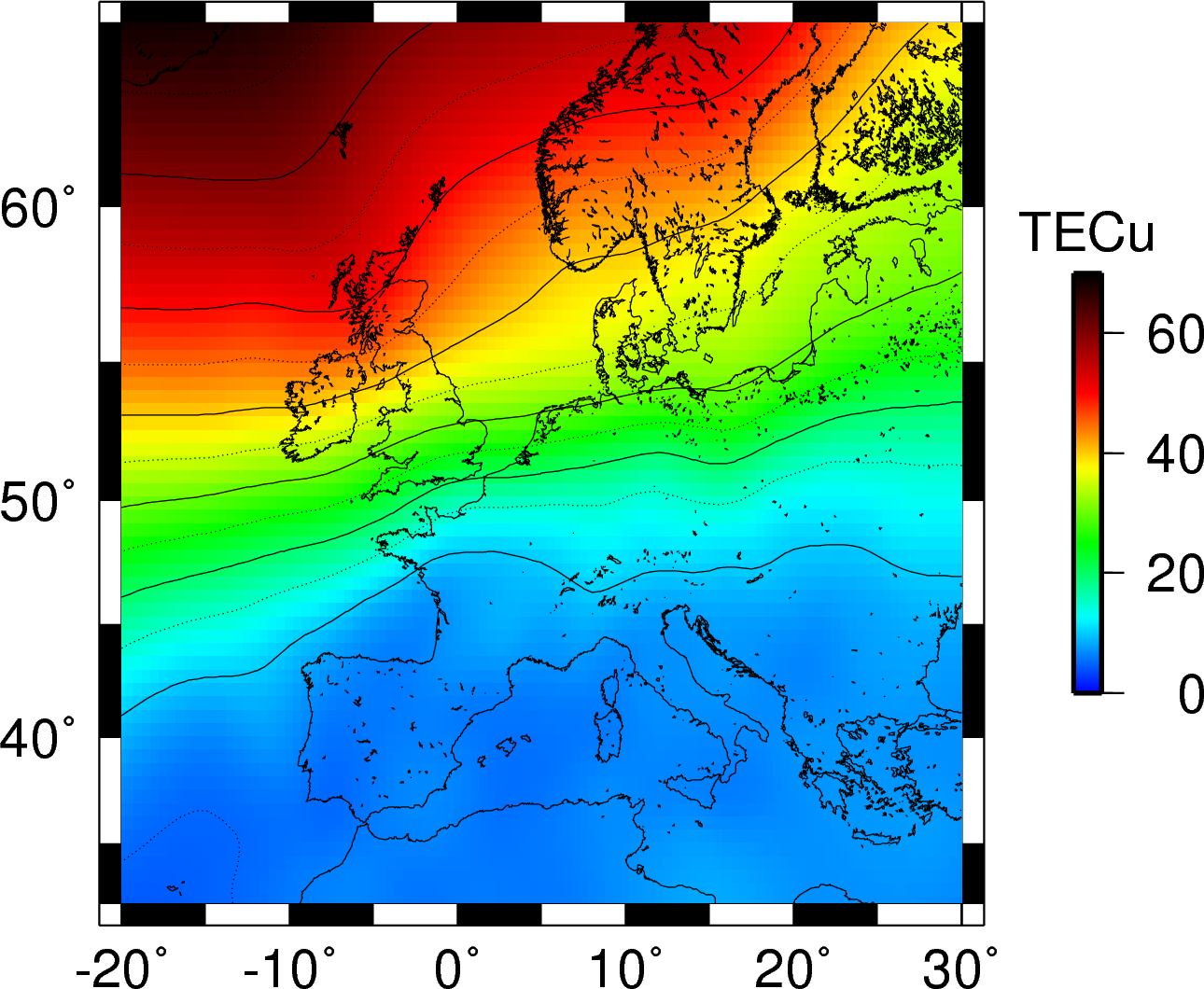
Figure 10: VTEC map during the Halloween storm (from 23:30 to 23:45 on 30 October 2003) extracted from the Near-Real Time products of ROB.
Figure 9 shows the VTEC behavior (in red) at three different locations above Europe (high-, mid- and low- latitudes) observed in Near-Real Time. The grey dots represent the normal ionospheric behavior expected based on the median VTEC from the 15 previous days. For example, the abnormal increase of VTEC above high latitude regions is concordant with the precision degradation of the position mentionned above.
Figure 10 shows the VTEC map above Europe estimated in Near-Real Time between 23:30 and 23:45 UTC. In normal ionospheric conditions, the expected VTEC values are comprise between 1 and 7 TECu (< 1.1 m on L1) during the night. However, during this storm, values reached 70 TECu (11 m on L1).
Bibliography
[Bergeot et al., 2010] Impact of the Halloween 2003 ionospheric storm on kinematic GPS positioning in Europe. GPS Solutions, Vol. 15, issue 2, pp. 0-180, doi:10.1007/s10291-010-0181-9
[Bilitza and Reinisch, 2008] International reference ionosphere 2007: Improvements and new parameters,Advances in Space Research, Elsevier Vol. 42,n°4, p599-609
[Breit and Tuve, 1926] A test of the existence of the conducting layer, Physical Review, APS, Vol. 28, n°3, p554-575
[Bust and Mitchell,2008] History, current state, and future directions of ionospheric imaging, Rev. Geophys., 46, RG1003, doi:10.1029/2006RG000212
[Hochegger et al., 2000] A family of ionospheric models for different uses, Physics and Chemistry of the Earth, Part C, Elsevier Vol. 25,n°4, p307-310
[Klobuchar, 1987] Ionospheric time-delay algorithm for single-frequency GPS users, IEEE Transactions on Aerospace and Electronic Systems, p325-331
[Kunitsyn and Tereshchenko, 2003] Ionospheric tomography. Springer, Berlin Heidelberg New York, 259p
[Rishbeth and Garriott] Introduction to ionospheric physics, New York, Academic Press, 1969. International geophysics series, Vol. 14
[Schaer et al., 1996] IONEX: The IONosphere map eXchange format version 1,Proceedings of the IGS Analysis Center Workshop, edited by JM Dow et al,p233-247
[Schuster, 1889] The Diurnal Variation of Terrestrial Magnetism, by Arthur Schuster and H. Lamb, Philosophical Transactions of the Royal Society of London, The Royal Society, p467-518.
[Stewart, 1961] On the Great Magnetic Disturbance of August 28 to September 7, 1859, as Recorded by Photography at the Kew Observatory. Proceedings of the Royal Society of London,Vol. 11, No. (1860 - 1862), p407-410.
More information in :
[Dach et al., 2007] Bernese GPS software version 5.0, Astronomical Institute, University of Bern, 612p
[Duquenne et al., 2005] GPS: localisation et navigation par satellites, Hermes, 330p
[Hofmann-Wellenhof et al., 2001] GPS theory and practice, New York, NY, 382p
[Liao, 2000] Carrier phase based ionosphere recovery over a regional area GPS network, Ph. D. dissertation, University of Calgary, 120p
[Schaer, 1999] Mapping and predicting the earth's ionosphere using the global positioning system, Ph. D. dissertation, University of Bern, Bern, Switzerland, 205p