Tropospheric Delay and GNSS Signals: Tutorial
Contents
2 Physical Modelling of the Tropospheric Delay
3 Modeling and Estimating the Tropospheric Propagation Delay
4 How To Estimate the Tropospheric Path Delays
5 Tropospheric Path Delay Products
6 A Little History
1. Introduction
The troposphere is the lower-most layer of the atmosphere and extends from the ground surface up to about 8km at the pole and up to about 17km at the equator. It contains about 75% of the total atmospheric mass and is primarily composed of nitrogen (78%), oxygen (20.9%) and argon (0.9%). The troposphere is the seat of all hydrometeors (rain, hail, snow...) and meteorological phenomena (clouds, weather fronts, cyclogenesis, thunderstorms...). The troposphere is a refractive medium, which influences the GNSS signals propagation. The troposphere induces an excess propagation path length on the GNSS signals, which varies from about 2.30m to 2.60m at sea level and can reach up to 50m for a satellite at an elevation angle of 3∘. About 90% of the tropospheric path delay stems from the dry atmosphere with typical values ranging from 2.25m to 2.35m at zenith. The atmospheric water vapour induces lower delays, which range typically between 0m and 0.40m. The dry tropospheric path delay depends mainly on the pressure and therefore it varies quite slowly in time (about 2cm per 12h) according to the pressure field variations. The wet tropospheric path delay depends on the water vapour distribution and changes much faster in both space and time. In addition, its variations are about three times as large as those in the dry component. Because of the high variability of the water vapour distribution in the atmosphere, it is considered to be one of the major error sources remaining in Space Geodesy.
2. Physical Modelling of the Tropospheric Delay
2.1 Refractive Index
The velocity of an electromagnetic wave in a medium depends of the refractive index, n, of the medium, which is defined by

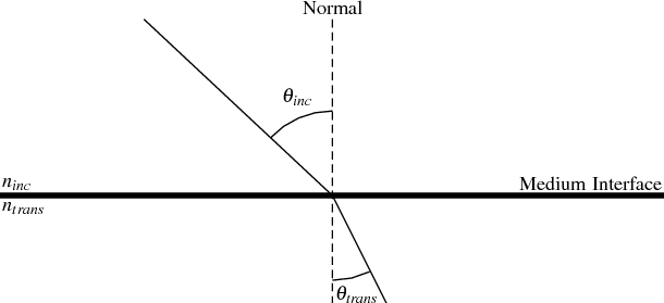
where c is the speed of light in vacuum and v is the speed of light in the corresponding medium. The refractive medium modifies not only the propagation velocity of the signal but also its direction of propagation. When a GNSS satellite signal hits the atmosphere at an incident angle other than the normal, the ray path is bent according to Snell’s law, which states

where ninc and ntran are the refractive indices of the incident and transmitted medium respectively (Figure 2.1). As the refractive index increases when descending towards the Earth, as the atmosphere becomes denser, the ray gradually bends more intensively. The troposphere is a non-dispersive medium, i.e. the refractive index n is independent of the signal frequency. Consequently, carrier-waves and Pseudo-Random-Noise (PRN) codes do propagate in it at the same speed.
2.2 Excess Propagation Path Length
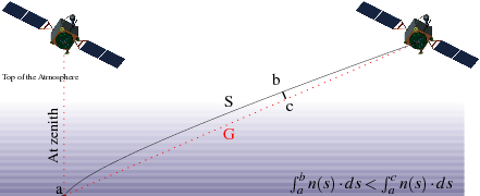
The excess propagation time, Δtph, of a radio-frequency signal is the difference between the time taken by the signal to traverse the refractive medium, having a refractive index n(s), and the time it would have taken in vaccum conditions. It reads

- S is the actual curved path of the radio-signal transmitted from a satellite to a receiver on the ground
- s is the curvilinear index along the actual signal path S
- G is the straight line distance (vacuum distance) that would have been the path without any atmosphere (vacuum conditions)
- vph is the phase velocity (although the group and phase velocities are roughly identical in the neutral atmosphere since the dispersion can be ignored at the frequencies transmitted by GNSS satellites)
- nph(s) is the refractive index along the signal propagation path S
- ϵ, α and c are respectively the elevation angle, the azimuth angle and the speed of light in vacuum
which gives in units of distance, the excess propagation path length:
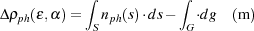
The first term in the equation above correspond to the "true" electrical path while the second term is the shortest geometrical path that the signal would have travelled in vacuum (Figure 2.2). It contains both the effect of the speed variation and the bending effect, which is usually neglected so that we can write
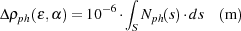
where Nph = 106 ⋅(nph-1) is the refractivity index.
2.3 Tropospheric Path Delays
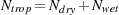
The troposphere consists of a mixture of different gases. The refractivity index of the tropospheric layer is thus the sum of the contribution of each constituent that composes the troposphere multiplied by its own density [Hall, 1979; Debye, 1929]. The total tropospheric refractivity index is usually divided into two parts named the "dry" (or hydrostatic) component and the "wet" (or non-hydrostatic) component, with the latter containing only the water vapour contribution:
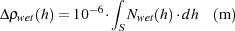
According to this decomposition, the total tropospheric path delay Δρtot can separated into the hydrostatic and non-hydrostatic (wet) tropospheric path delays, which read
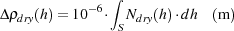
- Δρdry is the tropospheric hydrostatic path delay
- Δρwet is the tropospheric wet path delay
- h is the height above the mean sea level in meters
3. Modeling and Estimating the Tropospheric Propagation Delay
3.1 Slant Delays and Mapping Functions
In general, the radio-frequency signals recorded by a GNSS receiver do not arrive from the zenith direction but from slant directions. Tropospheric propagation delays depend on the actual path that the signals have to travel through the atmosphere and are therefore also functions of the satellite elevation angle. As illustrated in Figure 2.2, the lower to the horizon the GNSS satellite is, the bigger the portion of the atmosphere the signals will have to travel to reach the antenna’s receiver and, consequently, the higher the impact of the tropospheric refractivity on GNSS signals will be. To represent that, troposphere models include in general two parts: the first one is the a priori model for the tropospheric zenith path delay, which corresponds to the delay that would have a satellite at the zenith, and the second part is the mapping function, which account for the satellite elevation angle. The slant delay between the receiver A and the satellite k may be written, approximately, as the product of the tropospheric zenith path delay and the mapping function:

Over the past decades, Geodesists have developed a large variety of mapping functions to evaluate the delay experienced by microwave signals propagating through the neutral atmosphere at arbitrary elevation angles. The simplest mapping function that can be used is the cosecant of the elevation angle, mf(ϵ) = 1∕sin(ϵ), and is illustrated in Figure 3.1.
The mapping function is also generally different for the hydrostatic and wet tropospheric path delays, so that we can write

A plethora of mapping functions exist and may be found in the literature. The New Mapping Functions (NMF) proposed by Niell remain one of the most often used [Niell, 1996]. They are independent of any surface meteorological parameters. The two separated mapping functions for the hydrostatic and wet tropospheric delays. The NMF mapping functions can be used to elevation angles down to 3∘. Recent developments show possible improvements over these mapping functions by introducing, for example, atmospheric data from Numerical Weather Prediction (NWP) models. For the latest advanced mapping functions, the reader can refer to the Vienna Mapping Function (VMF) and the Global Mapping Function (GMF) described in [Boehm et al., 2006].
3.2 A Priori Tropospheric Models
In most cases, the zenith a priori tropospheric model requires some input parameters, e.g., pressure, temperature and humidity. The values of these parameters may be derived either from a standard model of the atmosphere or from real meteorological observations.
3.2.1 Zenith Hydrostatic Tropospheric Delay Models
For the hydrostatic component of the tropospheric delay, two main a priori models (to be used along with the NMF) exist. They are the Saastamoinen [Saastamoinen, 1972] and the Hopfield [Hopfield, 1969b] models. We give here the expression for the hydrostatic a priori model developed by Saastamoinen. The model of Saastamoinen assumes that the dry atmosphere is in hydrostatic equilibrium. Based on the approximations presented in [Saastamoinen, 1972] and in [Davis et al., 1985] the final expression for the Zenith Hydrostatic Delay (ZHD) can be written as
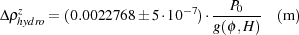
where P0 is the total ground pressure (in hPa) and the function g(ϕ,H) = (1-0.00266⋅cos(2ϕ)-2.8⋅10-7 ⋅H) is used to model the variations of the acceleration due to the gravity in function of the latitude ϕ (in degree) and the altitude of the station (in metre). More details on the Saastamoinen and Hopfield models can be found in [Saastamoinen, 1972; Davis et al., 1985; Kleijer, 2004; Elgered et al., 1991; Dejong, 1991; Hopfield, 1969a,b, 1971a] and [Hopfield, 1971b].
3.2.2 Zenith Wet Tropospheric Delay Models
Since the water vapour profile is difficult to obtain using only ground-based measurements of the temperature, pressure and humidity, the wet tropospheric delays remains usually unsatisfactory estimated by any a priori model, especially when high accuracy positioning and tropospheric parameters are targeted. Therefore, it is advised to only include an a priori model for the hydrostatic component and to account for the non-hydrostatic part by estimating the so-called site specific tropospheric parameters (see section 3.3).
3.3 Site Specific Troposphere Parameters
In high-accuracy GNSS applications, the residual tropospheric errors remaining after the application of only the a priori hydrostatic tropospheric models and its associated mapping function are too large to reach the requested positioning accuracy and these errors must be corrected. Therefore, we usually estimate what we call site-specific troposphere parameters based on the GNSS observations. These parameters are station and time dependent.
3.4 Azimuth Asymmetries and Gradient Parameters
When using low elevation angle observations, the azimuth asymmetry of the local troposphere gets more and more important and must be accounted for [Beutler et al., 2007]. Estimating horizontal tropospheric gradients is a common way to cope with these asymmetries and the station coordinate repeatability may be considerably improved by this measure as shown in [Rothacher et al., 1997] and [Meindl et al., 2004]. For more details on gradient parameter estimations we refer the reader to [Meindl et al., 2004] and [Kleijer, 2004].
3.5 Final Form of GNSS Tropospheric Models
The general mathematical form of a tropospheric model used in high-accuracy GNSS processing can be expressed as follow:

- t is the observation time
- zAk, αAk stand respectively for the zenith and azimuth angles of the satellite k observed from the station A
- ΔρAk is the true tropospheric path delay between the station A and the satellite k
- Δρapr,A(zAk) ⋅f(zAk) is the slant delay according to an a priori model and its mapping function
- ΔhρA(t), f(zAk) is a (time-dependent) site specific zenith path delay parameter and its associated mapping function
- ΔnρA(t), ΔeρA(t) are the (time-dependent) horizontal north and east troposphere gradient parameters
4. How To Estimate the Tropospheric Path Delays
Once the station coordinates have been precisely determined, ionosphere-free carrier-phase double-differences (add link to the proper tutorial) can be used, while fixing the coordinate, to estimate the tropospheric zenith path delay for each GNSS station using the model presented above.
5. Tropospheric Path Delay Products
Once estimated during the GNSS observation analysis, the tropospheric zenith path delay can be re-used for positioning or third party applications as a correction. The tropospheric zenith path delay estimated can also be used in meteorology (see EUMETNET - E-GVAP in the project section). Two types of product can be generated: tropospheric zenith path delay time series, which are used in NWP models, and tropospheric zenith path delay maps, which are used in nowcasting applications. Need to add a TS and a graph
6. A Little History
- 1969: Hopfield proposed an a priori tropospheric zenith path delay model using surface meteorological records, i.e. the pressure, the temperature and the relative humidity in [Hopfield, 1969a]
- 1972: Marini proposed the continued fraction form mapping function to map the tropospheric zenith path delay delay at any elevation angle in [Marini, 1972]
- 1972-1973: Saastamoinen proposed his own a priori tropospheric zenith path delay model using pressure, temperature and relative humidity surface observations in [Saastamoinen, 1972, 1973]
- 1996: Niell proposed his New Mapping Functions (NMF) based on a 3-term truncation of the continued fraction form mapping function of Marini in [Niell, 1996]
- 2000: Niell proposed his Isobaric Mapping Functions (IMF), which make use of the output of global Numerical Weather Prediction (NWP) models in [Niell, 2000]
- 2004: Boehm and Schuh proposed their Vienna Mapping Functions (VMF) based on a 3-term truncation of the continued fraction form of Marini where the coefficients are obtained from the ECMWF NWP model output in [Boehm and Schuh, 2003, 2004]. The VMF is to be used along with the Vienna Zenith Hydrostatic Delay (VZHD) provided directly from ray tracing through the NWP model grid
- 2006: Boehm et al. proposed their Global Mapping Functions (GMF) based on a 3-term truncation of the continued fraction form of Marini where the coefficients were obtained from the ECMWF 40-year re-analysis data (ERA40) in [Boehm et al., 2006; Uppala et al., 2005]. The GMF is to be used along with the Global Pressure Temperature (GPT) ZHD provided from the ERA40 re-analysis
Bibliography
[Beutler et al., 2007]
Beutler, G., Bock, H., Dach, R., Fridez, P., Gäde, A., Hugentobler, U., Jäggi, A.,
Meindl, M., Mervart, L., Prange, L., Schaer, S., Springer, T., Urschl, C., and Walser,
P. 2007.
Bernese GPS Software Version 5.0
Astronomical Institute, University of Bern.
[Boehm and Schuh, 2003]
Boehm, J. and Schuh, H. 2003.
Vienna Mapping Functions.
In Proceedings of the 16th Working Meeting on European VLBI for Geodesy and Astronomy, pages 131–143. verslag des Bundesamtes für Kartographie und Geodaesie.
[Boehm and Schuh, 2004]
Boehm, J. and Schuh, H. 2004.
Vienna mapping functions in VLBI analysis.
In Geophysical Research Letter, 31(L01603, doi: 10.1029/2003GL018984).
[Boehm et al., 2006]
Boehm, J., Werl, B., and Schuh, H. 2006.
Troposphere Mapping Functions for GPS and Very Long Baseline Interferometry from European Centre for Medium-Range Weather Forecasts Operational Analysis Data.
In Journal of Research Letter, 111(B02406, doi: 10.1029/2005JB003629).
[Davis et al., 1985]
Davis, J. L., Herring, T. A., Shapiro, I. I., Rogers, A. E. E., and Elgered, G. 1985.
Geodesy by radio interferometry: effects of atmospheric modelling errors on estimates of baseline length.
In Radio Science, 20(6):1593–1607.
[Debye, 1929]
Debye, P. 1929.
Polar molecules
Dover, New York.
[Dejong, 1991]
Dejong, C. D. 1991.
GPS: Satellite orbits and atmospheric effects.
In NASA STI/Recon Technical Report N, 92:14097–+.
[Elgered et al., 1991]
Elgered, G., Davis, J. L., Herring, T. A., and Shapiro, I. I. 1991.
Geodesy by Radio Interferometry: Water Vapor Radiometry for Estimation of Wet Delay.
In Journal of Geophysical Research, 96(B4):6541–6555.
[Hall, 1979]
Hall, M. P. 1979.
Effects of the troposphere on radio communication.
Peter Peregrinus LTD on behalf of the Institution of Electrical Engineers.
[Hopfield, 1969a]
Hopfield, H. S. 1969.
Approximation to the tropospheric range correction.
In Applied Physics Laboratory, pages 572 – 569. Silver Spring, Md., 12. November, S1A-572-69, 4 pp.
[Hopfield, 1969b]
Hopfield, H. S. 1969.
Two-quartic tropospheric refractivity profile for correcting satellite data.
In Journal of Geophysical Research, 74(18):4487–4499.
[Hopfield, 1971a]
Hopfield, H. S. 1971.
Tropospheric effect on electromagnetically measured range: Prediction from surface weather data.
In Radio Science, 6(3):357 – 367.
[Hopfield, 1971b]
Hopfield, H. S. 1971.
Tropospheric range error at the zenith.
Presented at Fourteenth Plenary Meeting of the Committee on Space Research, Seattle, Washington, 17 June-2 July, June, 31 pp.
[Kleijer, 2004]
Kleijer, F. 2004.
Troposphere Modeling and Filtering for Precise GPS Leveling.
Ph.D. thesis, Delft University of Technilogy.
[Marini, 1972]
Marini, J. W. 1972.
Correction of satellite tracking data for an arbitrary tropospheric profile.
In Radio Science, 7(2):223–231.
[Meindl et al., 2004]
Meindl, M., Schaer, S., Hugentobler, U., and Beutler, G. 2004.
Tropospheric Gradient Estimation at CODE: Results from Global Solutions, in Applications of GPS Remote Sensing to Meteorology and Related Fields.
In Journal of the Meteorological Society of Japan, 82(1B):331 – 338.
[Niell, 1996]
Niell, A. E. 1996.
Global mapping functions for atmosphere delay at radio wavelength.
In Journal of Geophysical Research, 101(B2):3227–3246.
[Niell, 2000]
Niell, A. E. 2000.
Improved Atmospheric Mapping Functions for VLBI and GPS.
In Earth Planets Space, 52:699–702.
[Rotacher et al., 1997]
Rothacher, M., Springer, T. A., Schaer, S., and Beutler, G. 1997.
Processing Strategies for Regional GPS Networks.
In Springer, editor, Proceedings of the IAG General Assembly in Rio, September, 1997
[Saastamoinen, 1972]
Saastamoinen, J. 1972.
Atmospheric correction for troposphere and stratosphere in radio ranging of satellites. The Use of Artificial Satellites for Geodesy.
In Papers presented at the Third International Symposium on The Use of Artificial Satellites for Geodesy, Eds. S. W. Henriksen, A. Mancini, B. H. Chovitz, AGU,
AIAA, NOAA, U.S.ATC, Washington, D. C., 15-17 April 1971, American Geophysical Union, Washington, D. C., Geophysical monograph 15, pages 247 – 252.
[Saastamoinen, 1973]
Saastamoinen, J. 1973,
Contributions to the theory of atmospheric refraction, part II.,
In Bull. Geod., 107:13–34.
[Uppala et al., 2005]
Uppala, S. M., KAllberg, P. W., Simmons, A. J., Andrae, U., Bechtold, V. D. C.,
Fiorino, M., Gibson, J. K., Haseler, J., Hernandez, A., Kelly, G. A., Li, X., Onogi,
K., Saarinen, S., Sokka, N., Allan, R. P., Andersson, E., Arpe, K., Balmaseda,
M. A., Beljaars, A. C. M., Berg, L. V. D., Bidlot, J., Bormann, N., Caires, S.,
Chevallier, F., Dethof, A., Dragosavac, M., Fisher, M., Fuentes, M., Hagemann, S.,
Hólm, E., Hoskins, B. J., Isaksen, L., Janssen, P. A. E. M., Jenne, R., McNally,
A. P., Mahfouf, J.-F., Morcrette, J.-J., Rayner, N. A., Saunders, R. W., Simon, P.,
Sterl, A., Trenberth, K. E., Untch, A., Vasiljevic, D., Viterbo, P., and Woollen, J.
2005,
The ERA-40 re-analysis,
In Quarterly Journal of the Royal Meteorological Society, 131:2961–3012.